Using Big Data for understanding churn in the music streaming industry

Introduction

Which song have you been listening to lately? Did you enjoy the experience on your music app? Or you had a hard time finding your favorite song?

Regardless of the type of music you like or the app you use, we, in general, create a lot of events while streaming music, whether on an app or in our browser. Events like visiting a page, clicking the play button, going through settings finding your artist, adding your best friend to share that nostalgic song. Events like these create an enormous amount of data.

While music services try their best to keep their customers happy, sometimes misfortune happens and customers do churn. In such scenarios, the data we created is the trail we left which can come in handy in understanding the problem or even finding similar behavior in other users.

Just as electricity transformed almost everything 100 years ago, today I actually have a hard time thinking of an industry that I don’t think AI will transform in the next several years. - Andrew Ng

With that being said, let’s try predicting churn from a music streaming dataset. Since the dataset is a 12 GB user log file, we will perform analysis on a relatively smaller size data(~128 MB) and use the insights to train on the bigger data. The data for these analyses and modeling is provided by Udacity.

In this blog post, I will be using pyspark for tackling this problem. Since we are essentially predicting churn, which takes binary value, we can take it as a classification problem. I will be training various models like RandomForestClassifier, LogisticRegression, GBTClassifier, NaiveBayes and DecisionTreeClassifier. These are a few classification model pyspark provides. In this process, I will go through 6 common phases of model development. The phases are:

1. Data Understanding
2. Business Understanding
3. Exploratory Data Analysis
4. Feature Engineering
5. Modeling
6. Evaluation

Data Understanding

Looking at the data, the data set is a single user log file containing 18 columns. We can easily show these columns using pyspark printSchema() method.

root
 |-- artist: string (nullable = true)
 |-- auth: string (nullable = true)
 |-- firstName: string (nullable = true)
 |-- gender: string (nullable = true)
 |-- itemInSession: long (nullable = true)
 |-- lastName: string (nullable = true)
 |-- length: double (nullable = true)
 |-- level: string (nullable = true)
 |-- location: string (nullable = true)
 |-- method: string (nullable = true)
 |-- page: string (nullable = true)
 |-- registration: long (nullable = true)
 |-- sessionId: long (nullable = true)
 |-- song: string (nullable = true)
 |-- status: long (nullable = true)
 |-- ts: long (nullable = true)
 |-- userAgent: string (nullable = true)
 |-- userId: string (nullable = true)

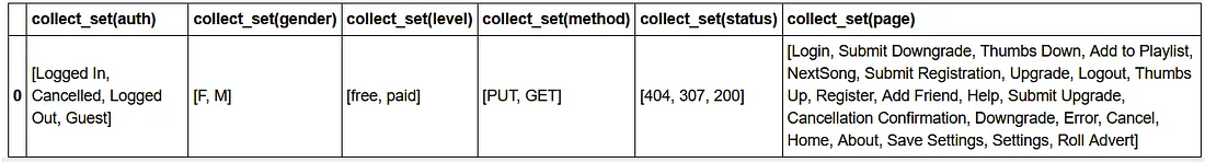
Quickly going through the schema and dataset, we can see there are some categorical as well as numerical columns. Auth, gender, level, method, status, page, and userAgent are some of the categorical columns while length( length of the song played), itemInSession, SessionId are some of the numerical columns.

On displaying the distinct values in these categorical columns we can see that we have a lot of pages like Login, Logout, NextSong, Home, About, Error, Thumbs Up, etc. Users can trigger events by visiting these pages. Along with that other details of users are also captured in the event such as user details, level(subscription status), status(HTTP code), method(HTTP method); and auth and device used to access the page as well as time.

Distinct values of some categorical variables

Defining Churn

A User churns when they leave a platform or simply stop using the services. While losing a single user might not be of any concern but losing consistently is of grave concern to any business. In this example, we can take canceling a subscription as a churn. In order to cancel a subscription, the user must visit the page ‘Cancellation Confirmation’ and that is our cue. Any user is marked as churn if in future or in past (for our dataset), has canceled subscription, say churn event, i.e. triggered event Cancellation Confirmation.

Business Understanding

After looking at the data, we can ask some basic questions before we proceed.

1. What is the effect of different user-page interactions on their churn status?
2. Does the gender, devices used and status 404( an error) code affect the user churn status?
3. How do active days, total sessions, minutes of play, number of songs play affect the churn status?

Exploratory Data Analysis

User-page interaction

As we have tagged churn, it would be interesting to see what pages users have visited based on their churn status.

Page visits box plot of users by their churn status

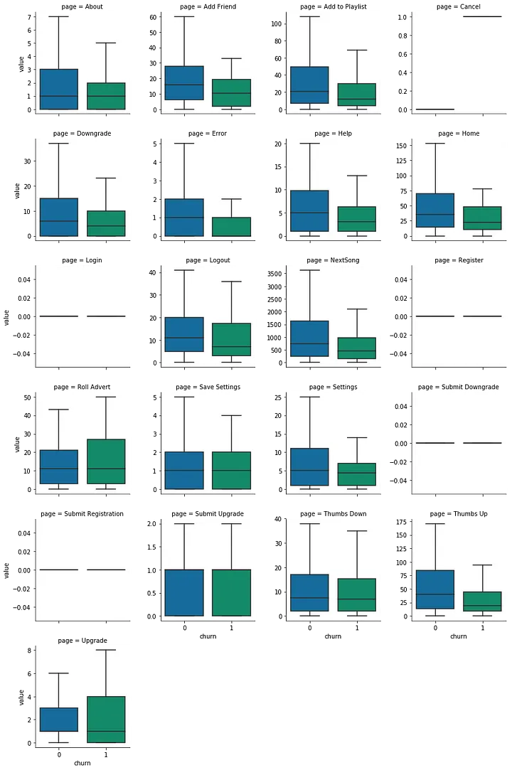
Through these box plots, we can see the significant differences in both groups by looking at mean, interquartile range, and spread.

• The churned group are less likely to visit pages: About, Add Friend, Add to Playlist, Downgrade, Error, Help, Home, NextSong, Settings, and Thumbs Up.
• And more likely to visit: Roll Advert, Upgrade

Affect of gender, devices used and status 404 faced on churn

User attributes and device used box plot by their churn status

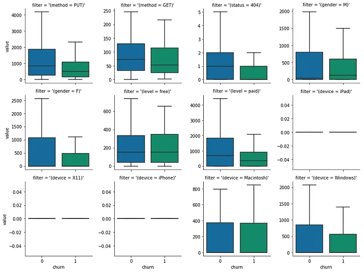
From these plots we can see that:

• put method is used by non-churned users more.
• The GET method is almost the same among both groups.
• status 404 is hit more by non-churned users.
• Male users are more prone to churn than female users.
• Paid users are less likely to churn.
• There is a variation for windows device users

How do active days, total sessions, minutes of play, number of songs play affect the churn status?

User activities box plot by their churn status

From these plots we can see that:

• fewer sessions are created by churned users.
• fewer songs are played by churned users.
• consequently less total playtime of churned users.
• also, the churn users have fewer items in a session.
• there is a lot of variation in the song length of churn users.
• active days is very low for churn users.
• overall the activity/interaction with key features is less for churned users.

Feature Engineering

Based on the analysis, we can add 3 sets of features:

1. Page-interaction features — count of different page visits
2. Key activities interaction features — song play duration, sessions, and other key activities
3. User attributes — devices used for interaction, status code

Here is the summary of features used:

1. Page-interaction features
    - about page visit count
    - add friend visit count
    - Add to playlist visit count
    - Downgrade page visit count
    - Error page visit count
    - home page visit count
    - roll advert count
    - help page visit count
    - settings page visit count
    - thumps up count
    - Upgrade count
2. Key activities interaction features
    - total_sessions
    - number of songs played
    - total time spent playing songs
    - maximum number of activity in a session
    - average length of song played
    - active days on the platform
    - average number of song played per session
    - songs played in free tier
    - songs played in paid tier
3. User attributes
    - faced 404 status code
    - weather PUT method used
    - device used

1. Page-interaction features

User page interaction is essential in understanding the user churn. From the page event, we can count the page-visit by each user. This could be essential as for e.g. a higher count of ‘Thumbs Up’ page visits might signal towards a long-term customer. Below code, snippet calculates just that only.

def calc_page_visit_features(df):
    """ calculation of page visit count features
        Input: 
            df - event dataframe with page and userId
        Output:
            page_visit_features: page visit feature by each user
    """
    page_visit_features = df.groupby("userId")\
        .pivot("page")\
        .count()\
        .fillna(0)\
        .select("userId", 
              "About", 
              "Add Friend", 
              "Add to Playlist", 
              'Downgrade', 
              'Error', 
              'Help', 
              'Home', 
              'Roll Advert', 
              'Settings', 
              'Thumbs Up', 
              'Upgrade')
    return page_visit_features

2. Key activities interaction features

Since we are doing analysis on music streaming data, playing songs, creating multiple sessions, longer session activities can be precious in identifying churn. We can calculate the features by grouping users and aggregating these metrics. The code for it is given below:

def calc_activity_feature(df):
    """ calculation of key activity features
        Input: 
            df - event dataframe
        Output:
            key_activity_features: key_activity_features of each user
    """
    activity_feature = df.groupby("userId")\
        .agg(F.countDistinct("sessionId").alias("total_sessions"), 
             F.sum(F.when(F.col("page") == "NextSong", 1).otherwise(0)).alias("number_of_song_played"),
             F.sum("length").alias("total_time_played"),
             F.expr("max(distinct(sessionId, itemInSession).itemInSession) as max_session_item"),
             F.mean("length").alias("avg_song_length"),
             ((F.max("ts")-F.min("ts"))/(24*60*60*1000)).alias("active_days")
            )\
        .withColumn("songs_per_session", F.col("number_of_song_played")/F.col("total_sessions"))
    
    
    free_song_played = df.filter(F.col("page")=="NextSong")\
                        .filter(F.col("level")=="free")\
                        .groupby("userId").count()\
                        .withColumnRenamed("count", "free_song_played")
    
    paid_song_played = df.filter(F.col("page")=="NextSong")\
                        .filter(F.col("level")=="paid")\
                        .groupby("userId").count()\
                        .withColumnRenamed("count", "paid_song_played")
    
    key_activity_features = activity_feature\
                                .join(free_song_played, "userId")\
                                .join(paid_song_played, "userId")\
                                .fillna(0)
    
    return key_activity_features

3. User attributes

Lastly, users’ attributes like the device they are using, errors they are facing while streaming can have a significant impact on their experience. We can capture these by filtering such data and counting such occurrences. Again the code is given below for this:

def pivot_table_on_filter(df, filters):
    """ calculates count of event after applying each filter
        Input: 
            df - event dataframe
            filters - list of filters to be used on df
        Output:
            filtered_event_count: filtered event count of each user
    """
    new_columns = [F.sum(F.when(f, F.lit(1)).otherwise(0)).alias(str(f).strip("Column<b'( )'>")) for f in filters]
    
    filtered_event_count = df\
        .groupby("userId")\
        .agg(*new_columns)\
        .fillna(0)
    
    return filtered_event_count

def calc_device_features(df):
    """ calculation of device feature, method used and 404 status features
        Input: 
            df - event dataframe
        Output:
            device_features: device features of each user
    """
    filters = [F.col("method")=='PUT',
               F.col("status")==404,
               F.col("device")=='iPad', 
               F.col("device")=='X11', 
               F.col("device")=='iPhone',
               F.col("device")=='Macintosh',
               F.col("device")=='Windows',
              ]

    device_features = pivot_table_on_filter(df, filters)

    device_columns = ['device = iPad', 'device = X11', 'device = iPhone', 'device = Macintosh', 'device = Windows']
    for col in device_columns:
        device_features = device_features.withColumn(col, F.when(F.col(col) > 0, F.lit(1)).otherwise(F.lit(0)))

    return device_features

Modeling

After the feature creation is done, we can move to the model part. Here I have tried 5 models from pyspark ml module. I have used pyspark ml pipeline for convenience purposes.

# Create vector from feature data
feature_names = features.drop('label', 'userId').columns
vec_asembler = VectorAssembler(inputCols = feature_names, outputCol = "features")

# Scaling features
scalar = MinMaxScaler(inputCol="features", outputCol="scaled_features")

# definining classifiers
dt = DecisionTreeClassifier(labelCol="label", 
                            featuresCol="scaled_features")
rf = RandomForestClassifier(featuresCol="scaled_features", labelCol="label",
                                numTrees = 40,  featureSubsetStrategy='sqrt')
lr = LogisticRegression(featuresCol="scaled_features", labelCol="label", 
                        maxIter=20, regParam=0.02)
gbt = GBTClassifier(featuresCol="scaled_features", labelCol="label")
nb = NaiveBayes(smoothing=1.0, modelType="multinomial")

# Constructing Pipelines
pipeline_dt = Pipeline(stages=[vec_asembler, scalar, dt])
pipeline_rf = Pipeline(stages=[vec_asembler, scalar, rf])
pipeline_lr = Pipeline(stages=[vec_asembler, scalar, lr])
pipeline_gbt = Pipeline(stages=[vec_asembler, scalar, gbt])
pipeline_nb = Pipeline(stages=[vec_asembler, scalar, nb])

pipelines = [('decision Tree', pipeline_dt),
             ('random forest', pipeline_rf), 
             ('logistic regression', pipeline_lr),
             ('gradient boosting tree', pipeline_gbt),
             ('naive bayes', pipeline_nb)]

Now that we have our pipeline ready, we can fit our models.

fitted_models = [(name, pipe.fit(training)) for name, pipe in pipelines]

Results

The modeling part does take a quite amount of time to finish. After that is done we can move to the model evaluation stage.

Model Evaluation and Validation

In churn prediction, we need to take care of 2 important things: false positives and false negatives. In other words, our precision and recall should be high. Since the F1 score is the harmonic mean of the two, we can choose it as an evaluation metric. The below function can be used for evaluation on our fitted_models.

def evaluate_model(model, metric_name, test_data):
    """ Evaluation of model performance
        Input: 
            model - fitted model pipeline which can transform data
            metric_name - the metric to be used for model evaluation
            test_data - data/feature for the test set
        Output:
            score: the metric value on test_data
    """
    evaluator = MulticlassClassificationEvaluator(metricName = metric_name)
    predictions = model.transform(test_data)
    score = evaluator.evaluate(predictions)
    
    return score

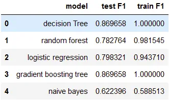
On evaluating our models on the test as well as the train set, we can see

• The Decision Tree and Gradient boosting method have the same accuracy.
• Logistic regression has an average f1 score.
• While naive Bayes is suffering a lot in terms of F1 score.
• Gradient boosting method is giving the better result of 0.87 f1 scores,

The model result on train and test set

Limitations

Gradient boosting algorithms are best for a varieties of regression and classification problems, but they have limitations two.

• After evaluating we can see that F1 on train score is 1 for GBT i.e. GBT Models will continue improving to minimize all errors. This can overemphasize outliers and cause overfitting. Here we need to regularize model and check for any over-fittings.
• Training time for GBT models are quite high even for small number of trees.

Grid search

Since we have clear winner, we can try improving accuracy using grid search. In pyspark, we can easily do model-tuning: using:

1. ParamGridBuilder — makes a grid of parameters for search space.
2. CrossValidator — trains and evaluate model(estimator) on various values on the search space.

I have decided to tune the max depth (Max number of levels in each decision tree) of gbt model with 3 fold cross-validation method.

# creating param grid for gbt model
param_grid = ParamGridBuilder()\
                .addGrid(gbt.maxDepth, [int(x) for x in np.linspace(start = 3, stop = 7, num = 3)]) \
                .build()

# model evaluator with F1 score as metric
model_evaluator = MulticlassClassificationEvaluator(metricName = 'f1')

# initializing cross validator with paramgrid, model pipline and model_evaluator
crossval = CrossValidator(estimator=pipeline_gbt,
                          estimatorParamMaps=param_grid,
                          evaluator=model_evaluator,
                          numFolds=3)

# fitting model on train data
cv_model = crossval.fit(training)

# calculating the F1 score on test data
metric = evaluate_model(cv_model, 'f1', test)
print(f" F1 Score from cross validation: {metric}")

# best cv model
best_model_pipeline = cv_model.bestModel

# best model
best_model = best_model_pipeline.stages[-1]
print('maxDepth - ', best_model.getOrDefault('maxDepth'))

F1 Score from cross validation: 0.8696581196581197
maxDepth -  3

After grid search F1 score was found to be 0.8696581196581197 and maxDepth to be 3.

Feature Importance

From our evaluation, we can see that gbt model has the best F1 score. Pyspark’s GBTClassifier has an attribute to get feature importance. According to its documentation: ‘Each feature’s importance is the average of its importance across all trees in the ensemble The importance vector is normalized to sum to 1. This method is suggested by Hastie et al. (Hastie, Tibshirani, Friedman. “The Elements of Statistical Learning, 2nd Edition.” 2001.) and follows the implementation from scikit-learn.’

Using this we can calculate the feature importance scaled to 1.

# feature importance
importances = best_model.featureImportances

# making feature importance dataframe
feature_importance = pd.DataFrame({'Importance': importances,
                                   'feature': feature_names})\
                        .sort_values(by = 'Importance', ascending = False)

sns.set(rc={'figure.figsize':(11, 4)})
sns.barplot(x="feature", y="Importance", data=feature_importance)
plt.xticks(rotation = 90)
plt.ylabel('Importance')
plt.xlabel('Feature')
plt.show()

Feature importance

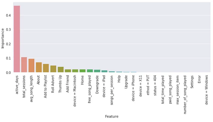
From the plot, we can see that active days, total sessions, average song length, about page visit count, etc were found to be the most important feature while the number of songs played, song played in the paid tier, Error page encountered count, device=Windows, etc, were found to be of least importance.

Improvement

• More features can be added to the model, like user artist interaction, or how many times a user has played a popular/trending song, or location-based feature like area to improve the metrics.
• Since we now know the most important features, we can try training on the subset of the total features sorted in descending order of importance. This will reduce time and should get the same metric. It will also make the model lighter.
• We can also try different model like Xgboost. Spark with scala has distributed xgboost API , but no such support is there for pyspark API yet. Still there are work around like this, this post. explain how to try it.

Conclusion

In this article, we have developed pyspark model for customer churn prediction in the music streaming industry; here are some takeaways:

• Churn prediction is an important problem in the industry. It is not a surprise that old customers bring more revenue to a brand than new customers. Adding to that, acquiring a new customer is costlier. In this project, I have made a model for churn prediction of a music company, ‘Sparkify’ which provides music streaming services.
• On Trying with 5 different models, I have seen that the Gradient boosting method appears to work best as its f1 score is better than other options.
• From feature importance, we can see that active days, total sessions, average song length, about page visit count, etc are some of the important features in identifying customer churn.
• Pyspark ML is a very powerful tool for machine learning. It provides all the model, feature transformation we can use for various types of problem statements. Like sklearn, we can build pipelines here and do cross-validation. Thus, it provides an end-to-end model development lifecycle in a distributed way. This can be particularly useful if we have 100s of gigabytes of data.

Please find the link to the github repo here.

Journey

Signup for Weekly Blog Updates.

Thank you!

You have successfully joined our subscriber list.